Initial setup
// load the OpenMP library required by Ranx
#pragma cling add_include_path("/usr/lib/llvm-9/include/openmp")
#pragma cling load("libomp.so.5")

#include <vector>
#include <g3p/gnuplot>
#include <ranx/random>

size_t count = 100'000;
float binwidth = 1.0f;
float binstart = 0.0f;
std::vector<int> v1(count), v2(count), v3(count), v4(count);

g3p::gnuplot gp;
gp  ( "set border 31 linecolor '#555555'" )
    ( "set key textcolor '#555555' box lc '#555555'" )
    ( "set title tc '#555555'" )
    ( "set style line 101 lt 1 lc '#555555' dt '. '" )
    ( "set grid ls 101" )
    ( "set style line 1 lt 1 lw 4 lc '#204a87'" )
    ( "set style line 2 lt 1 lw 4 lc '#cc0000'" )
    ( "set style line 3 lt 1 lw 4 lc '#c88a00'" )
    ( "set style line 4 lt 1 lw 4 lc '#4e9a06'" )
    ("binwidth = %f", binwidth)
    ("binstart = %f", binstart)
    ("bin(x) = binwidth * floor((x - binstart) / binwidth) + binstart + binwidth/2.0")
    ("set title 'Distribution Histogram'")
    ("set xlabel 'X' tc '#555555'")
    ("set ylabel 'Frequency' tc '#555555'")
    ("set xrange [binstart:binstart + 100]")
    ("set yrange [0:*]")
;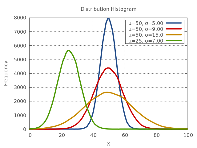
Normal distribution
Code
ranx::generate_n(std::begin(v1), count, ranx::bind(trng::normal_dist{50.0, 5.0},pcg32{}));
ranx::generate_n(std::begin(v2), count, ranx::bind(trng::normal_dist{50.0, 9.0},pcg32{}));
ranx::generate_n(std::begin(v3), count, ranx::bind(trng::normal_dist{50.0, 15.0},pcg32{}));
ranx::generate_n(std::begin(v4), count, ranx::bind(trng::normal_dist{25.0, 7.0},pcg32{}));
auto norm1 = make_data_block(gp, v1, 1);
auto norm2 = make_data_block(gp, v2, 1);
auto norm3 = make_data_block(gp, v3, 1);
auto norm4 = make_data_block(gp, v4, 1);

gp  << "plot"
    << norm1
    << "u (bin($1)):(1) title 'μ=50, σ=5.00' smooth kdensity w lines ls 1,"
    << norm2
    << "u (bin($1)):(1) title 'μ=50, σ=9.00' smooth kdensity w lines ls 2,"
    << norm3
    << "u (bin($1)):(1) title 'μ=50, σ=15.0' smooth kdensity w lines ls 3,"
    << norm4
    << "u (bin($1)):(1) title 'μ=25, σ=7.00' smooth kdensity w lines ls 4\n"
Output
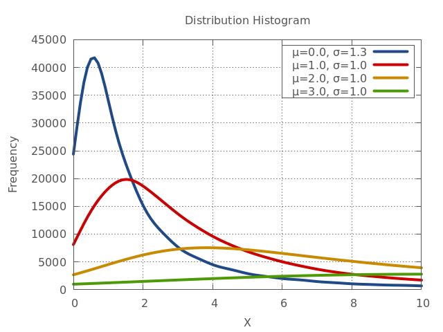
Log-normal distribution
Code
std::generate_n(std::begin(v1), count, std::bind(std::lognormal_distribution{0.0, 1.3},pcg32{}));
std::generate_n(std::begin(v2), count, std::bind(std::lognormal_distribution{1.0, 1.0},pcg32{}));
std::generate_n(std::begin(v3), count, std::bind(std::lognormal_distribution{2.0, 1.0},pcg32{}));
std::generate_n(std::begin(v4), count, std::bind(std::lognormal_distribution{3.0, 1.0},pcg32{}));
auto log_norm1 = make_data_block(gp, v1, 1);
auto log_norm2 = make_data_block(gp, v2, 1);
auto log_norm3 = make_data_block(gp, v3, 1);
auto log_norm4 = make_data_block(gp, v4, 1);

gp  << "set xrange [0:10]\n"
    << "plot"
    << log_norm1
    << "u (bin($1)):(1) title 'μ=0.0, σ=1.3' smooth kdensity w lines ls 1,"
    << log_norm2
    << "u (bin($1)):(1) title 'μ=1.0, σ=1.0' smooth kdensity w lines ls 2,"
    << log_norm3
    << "u (bin($1)):(1) title 'μ=2.0, σ=1.0' smooth kdensity w lines ls 3,"
    << log_norm4
    << "u (bin($1)):(1) title 'μ=3.0, σ=1.0' smooth kdensity w lines ls 4\n"
Output
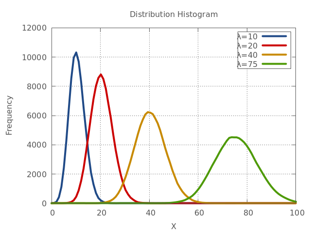
Poisson distribution
Code
std::generate_n(std::begin(v1), count, std::bind(std::poisson_distribution{10.0},pcg32{}));
std::generate_n(std::begin(v2), count, std::bind(std::poisson_distribution{20.0},pcg32{}));
std::generate_n(std::begin(v3), count, std::bind(std::poisson_distribution{40.0},pcg32{}));
std::generate_n(std::begin(v4), count, std::bind(std::poisson_distribution{75.0},pcg32{}));
auto poisson1 = make_data_block(gp, v1, 1);
auto poisson2 = make_data_block(gp, v2, 1);
auto poisson3 = make_data_block(gp, v3, 1);
auto poisson4 = make_data_block(gp, v4, 1);

gp  << "set xrange [0:100]\n"
    << "plot"
    << poisson1
    << "u (bin($1)):(1) title 'λ=10' smooth kdensity w lines ls 1,"
    << poisson2
    << "u (bin($1)):(1) title 'λ=20' smooth kdensity w lines ls 2,"
    << poisson3
    << "u (bin($1)):(1) title 'λ=40' smooth kdensity w lines ls 3,"
    << poisson4
    << "u (bin($1)):(1) title 'λ=75' smooth kdensity w lines ls 4\n"
Output