Embedding Plot Data

So far, we’ve used functions defined in Gnuplot for plotting. While it’s perfectly fine to use G3P to produce plots using pure Gnuplot facilities, as is usually the case, the whole point of using a language specific interface library like G3P is to plot data generated by C/C++ functions. There are two mechanisms for embedding data into a stream of Gnuplot commands and we’re going to explore them in the next two sections.

Inline data¶

If the special filename '-' appears in a plot command, then the lines immediately following the plot command are interpreted as inline data. To demonstrate that, let’s first define a function template:

Matlab’s Peaks

We use Matlab’s Peaks as our function:

F(x_1,x_2) = 3(1 - x_1)^2exp[-x_1^2 - (x_2 + 1)^2] - 10(\frac{1}{5}x_1 - x_1^3 - x_2^5)exp[-x_1^2 - x_2^2] - \frac{1}{3}exp[-(x_1 - 1)^2 - x_2^2]

(1)

Here’s the function template for the Matlab’s Peaks equation:

#include <cmath>

template<typename T>
auto matlab_peaks(T x1, T x2) -> T
{   return
    (   T(3)
    *   std::pow(T(1) - x1, T(2))
    *   std::exp(-std::pow(x1, T(2)) - std::pow(x2 + T(1), T(2)))
    -   (T(10) * (x1 / T(5) - std::pow(x1, T(3)) - std::pow(x2, T(5)))
    *   std::exp(-std::pow(x1, T(2)) - std::pow(x2, T(2))))
    -   (T(1) / T(3) * std::exp(-std::pow(x1 + T(1), T(2)) - std::pow(x2, T(2))))
    );
}

And here’s the code to produce a 3D plot:

#include <g3p/gnuplot>

g3p::gnuplot gp;

// setting our plot
gp  ("set nokey")
    ("set view 60, 320,,1.2")
    ("set border 895")
    ("unset colorbox")
    ("set grid x y z")
    ("set xrange[-3:3]")
    ("set yrange[-3:3]")
    ("set zrange[-8:10]")
    ("set ticslevel 0")
    ("set palette rgb 33,13,10")
    // ("set style line 101 lc 'black' lw 0.2")
    ("set pm3d depthorder border")
    // ("splot '-' with lines lc 'gray' lw 0.1");
    // ("splot '-' with pm3d ls 101");
    ("splot '-' with pm3d");
//           ^ --> tells gnuplot that data is coming after this command

// now we can start embedding our inline data...
for (float i = -3; i < 3; i += 0.15)
{   for (float j = -3; j < 3; j += 0.15) 
        gp << i << j << matlab_peaks(i, j) << "\n";
    gp.endl();
}

// once the data stream is finished we have to inform
// gnuplot by sending the end signal:
gp.end()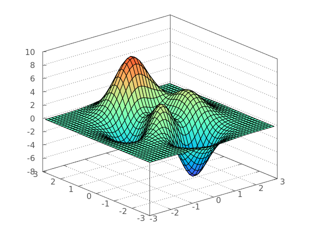

Datablocks¶

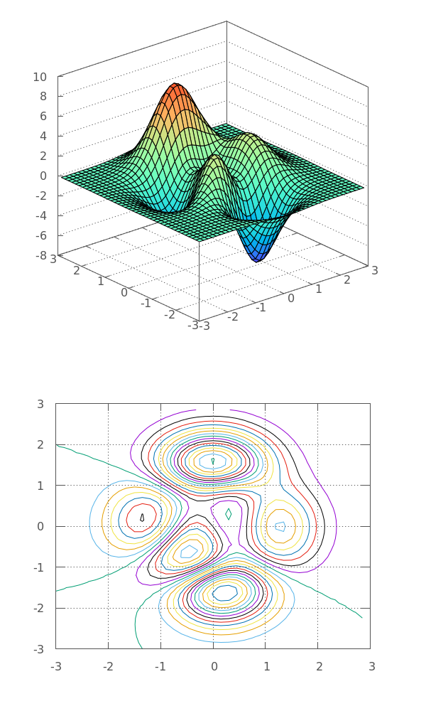
Data provided in the previous method can only be used once, by the plot command it follows. Often, we want to use the data referenced by more than one plot command in the same plot or multiplots. That’s where datablocks come into play. You just need to define the datablock once and then you can use its name to refer to it. Here is the multiplot of the same Peaks function using datablocks:

#include <vector>

// we first put our data in a 3d vector
std::vector<float> grid(40 * 40 * 3); // 40 x 40 x 3 grid
auto itr = std::begin(grid);
for (float i = -3; i <= 3; i += 0.15)
    for (float j = -3; j <= 3; j += 0.15)
    {   *itr++ = i;
        *itr++ = j;
        *itr++ = matlab_peaks(i, j);
    }

// we use make_data_block function provided by G3P
// to turn our vector into a datablock
auto peaks = make_data_block(gp, grid, 3, 40);

// now we can use it in a multiplot
// NOTE: we mix and match C and C++ conventions here...
gp  ("set term pngcairo size 600,1000")      // make some space for the 2nd plot
    ("set multiplot layout 2,1 spacing 0,0") // switch to multiplot
    << "splot" // start plotting as the rest has been already set
    << peaks   // <-- using peaks once
    << "with pm3d\n";
gp  ("set view map")
    ("set contour")
    ("set cntrparam levels 50")
    ("unset surface")
    << "splot"
    << peaks // <-- using peaks twice
    << "w lines\n"
    << "unset multiplot\n"