A Primer On Randomness

Overview¶

In the world around us, randomness is everywhere. But is it truly random? To answer that question, we need to know the sources of randomness.

Types of Randomness¶

Algorithmic Random Number Generators (ARNGs)¶

ARNGs are computer algorithms that can automatically create long runs of numbers with good random properties but eventually the sequence repeats. The first one developed by John von Neumann but it didn’t have a good quality.

Then a mathematician named D. H. Lehmer made good progress toward this idea by introducing Linear congruential generator. Despite being one of early ones, LCG’s have some characteristics that make them very suitable for parallel random number generation.

Under the hood of an ARNG¶

A typical algorithmic random number engine (commonly shortened to engine ) has three components:

• The engine’s state.
• The state-transition function (or Transition Algorithm, TA) by which engine’s state is advanced to its successor state.
• The output function (or Generation Algorithm, TG) by which engine’s state is mapped to an unsigned integer value of an arbitrary size.

Below, you can see all the above components in a super simple, super fast lehmer64’s engine:

__uint128_t g_lehmer64_state;               // <-- the engine's state

uint64_t lehmer64()
{   g_lehmer64_state *= 0xda942042e4dd58b5; // <-- the state-transition function
    return g_lehmer64_state >> 64;          // <-- the output function
}

We can easily transform the above engine into a working code by a simple modification:

// transform into a class with overloaded function operator
struct lehmer64
{   __uint128_t _lehmer64_state;
    lehmer64(__uint128_t seed = 271828ull) // e as the default seed
    :   _lehmer64_state(seed << 1 | 1)     // seed must be odd
    {}
    uint64_t operator() ()
    {   _lehmer64_state *= 0xda942042e4dd58b5;
        return _lehmer64_state >> 64;
    }
};

// instantiate an engine with the default seed...
lehmer64 e;

// get our first random number
e()

Important attributes of an ARNG¶

Now that we know the internals of an engine, it’s much easier to understand the important attributes of them:

Statistical analysis of ARNGs¶

Are the numbers that we got from lehmer64 really random? This question is surprisingly hard to answer. The practical approach is to take many sequences of random numbers from a given engine and subject them to a battery of statistical tests.

The first in a series of such tests was DIEHARD, introduced by George Marsaglia back in 1995. Followed by DIEHARDER by Robert G. Brown in 2006. And last but not least, TestU01 by Pierre L’Ecuyer and Richard Simard of the Université de Montréal back in 2007, which is considered as a gold standard.

TestU01 includes three subset:

• Small Crush (10 tests)
• Crush (96 tests)
• Big Crush (106 tests)

To be a good random number generator it is not sufficient to just “pass” Big Crush, but if it can’t pass Big Crush, there’s a problem with it.

Rest assured we’re not going to do Big Crush here for our engine! 😅 Nevertheless, we’ll check it with two simpler visual tests in the next sections.

Visual analysis with randogram¶

One way to examine a random number generator is to create a visualization of the numbers it produces, a so called randogram. Our eyes are very powerful pattern recognizers, and by looking at the randogram we can almost instantly detect any recognizable pattern.

We can use Gnuplot’s rgbimage plot style available in g3p::gnuplot to render such a randogram for our lehmer64 engine:

#include <g3p/gnuplot>

g3p::gnuplot gp;

int w = 200, h = 200;
gp  ("set term pngcairo size %d,%d", w, h)
    ("unset key; unset colorbox; unset border; unset tics")
    ("set margins 0,0,0,0")
    ("set bmargin 0; set lmargin 0; set rmargin 0; set tmargin 0")
    ("set origin 0,0")
    ("set size 1,1")
    ("set xrange [0:%d]", w)
    ("set yrange [0:%d]", h)
    ("plot '-' u 1:2:3:4:5 w rgbimage");
for (size_t i = 0; i < w; ++i)
    for (size_t j = 0; j < h; ++j)
    {   int c = e() % 256; // use modulo to bring it into 0-255 range
        gp << i << j << c << c << c << "\n";
    }
gp.end()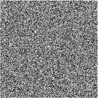

We can even monitor a longer sequence of random numbers by generating a white noise. Using one of the terminals in g3p::gnuplot that supports animation (e.g. gif or webp), we can easily transform our randogram into a white noise. There shouldn’t be any recognizable pattern either in the randogram or the white noise. Check here for an example of a failed randogram.

gp  ("set term gif enhanced animate size %d,%d", w, h);
for (size_t frame = 0; frame < 10; ++frame)
{   gp("plot '-' u 1:2:3:4:5 w rgbimage");
    for (size_t i = 0; i < w; ++i)
        for (size_t j = 0; j < h; ++j)
        {   int c = e() % 256;
            gp << i << j << c << c << c << "\n";
        }
    gp.end();
}
gp

Visual analysis with histogram¶

A good-quality ARNG, especially one generating numbers from a continuous uniform distribution, should produce a histogram that is approximately flat. This indicates that all possible values (or all bins) are occurring with roughly the same frequency, which is the definition of a uniform distribution.

The test requires a large sample size (e.g., 10⁵ or more numbers) to accurately reveal the underlying distribution. So, we use the lehmer64 to generate a long sequence of numbers within a specified range (e.g., [1, 100]) and divide the entire range of the generated numbers into a sufficient number of equal-sized bins and count how many of the generated numbers fall into each bin. Then, plot the bins on the x-axis and the counts on the y-axis.

Since Gnuplot introduced a specific bins data filter for generating histograms from raw data in version 5.2, we can either perform the bin processing in C++ and pass the bins, or pass the raw data to Gnuplot and do the processing there. To that end, we’ll use a g3p::gnuplot. Let’s start with the common settings for the two plots:

size_t count = 100'000;

g3p::gnuplot gp; // start with a new gnuplot instance

gp  ( "set border 31 linecolor '#555555'" )
    ( "set key textcolor '#555555' box lc '#555555'" )
    ( "set title tc '#555555'" )
    ( "set style line 101 lt 1 lc '#555555' dt '. '" )
    ( "set border lc '#555555'" )
    ( "set style fill solid 0.5" )
    ( "set grid ls 101" )
    ( "unset key; unset colorbox;" )
    ( "set title 'Distribution Histogram'" )
    ( "set ylabel 'Frequency' tc '#555555'" )

;

And here are both implementations and the resulting histograms in a tab so you can compare them in one place:

C++ bins

Gnuplot bins

#include <unordered_map>    // <-- std::unordered_map

// start with the same seed to get comparable results
lehmer64 e{};

// counting bins first
std::unordered_map<int, int> hist;
for (int i = 0; i < count; ++i)
    ++hist[e() % 100]; // use modulo to bring it into 0-100 range

gp  ( "set xrange [0:100]" )
    ( "set yrange [0:*]" )
    ( "plot '-' u 1:2 smooth frequency with boxes" );
    for (auto [x, y] : hist)
        gp << x << y << "\n";  
gp.end()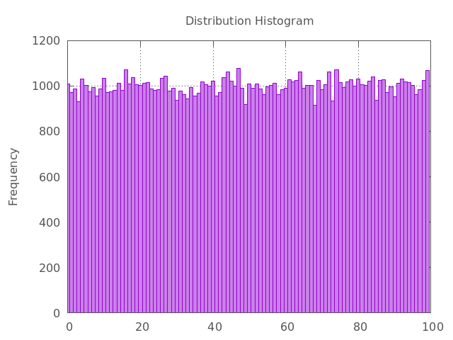

float  binwidth = 1.0f, binstart = 0.0f;

// start with the same seed to get comparable results
lehmer64 e{};


gp  ( "binwidth = %f", binwidth )
    ( "binstart = %f", binstart )
    ( "bin(x)=binwidth*floor((x-binstart)/binwidth) + binstart + binwidth/2.0" )
    ( "set boxwidth binwidth * 0.9" )
    ( "set xrange [binstart:binstart + 100]" )
    ( "set yrange [0:*]" )
    ( "plot '-' u (bin($1)):(1) smooth frequency with boxes" );
    for (size_t i = 0; i < count; ++i)
        gp << e() % 100 << "\n";  // use modulo to bring it into 0-100 range
gp.end()

We can also use the smooth kdensity option to plot a kernel density estimate using Gaussian kernels:

gp  ("plot '-' u (bin($1)):(1) smooth kdensity with lines lw 2.0");
for (size_t i = 0; i < count; ++i)
    gp << e() % 100 << "\n";
gp.end()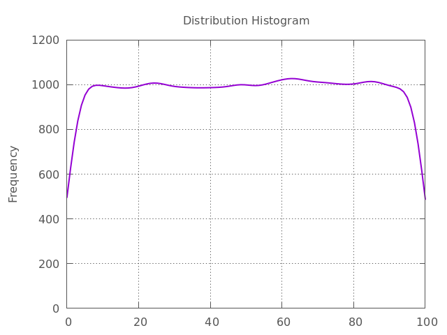

If the ARNG has flaws, the histogram will show significant peaks and valleys or a sloping/biased shape. This indicates that certain values or ranges are being generated more often than others, proving the numbers are not truly random and uniform.

Reproducibility vs. fair play¶

One last thing that we need to cover before going to the next chapter is the difference between reproducibility and playing fair. An ARNG must be reproducible. It means if you use them with the same seed and distribution, you should get the same sequence of numbers every time.

The latter statement is not necessarily true when you use them in a parallel region of a code. In parallel Monte Carlo simulations, playing fair means the outcome is strictly independent of the underlying hardware. That means you should get the same sequence independent of the number of parallel threads.